Working with results#

For all example code on this page, ospgrillage is imported as og

import ospgrillage as og

Extracting results#

After analysis, results are obtained using get_results().

all_result   = example_bridge.get_results()
patch_result = example_bridge.get_results(load_case="patch load case")

The first call returns results for every load case; the second filters to one.

What is an xarray Dataset?#

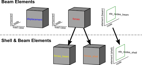
The returned object is an xarray Dataset — think of it as a multi-dimensional, labelled table. Rather than accessing data by integer index (row 3, column 7), you access it by name (Loadcase="Barrier", Component="Mz_i"). This makes result queries self-describing and much less error-prone.

The Dataset contains five named data variables:

Variable	Axes (dimensions)	Contents
`displacements`	Loadcase x Node x Component	Translations (x, y, z) and rotations (theta_x, theta_y, theta_z) at each node
`velocity`	Loadcase x Node x Component	Velocities (dx, dy, dz) and angular velocities (dtheta_x/y/z)
`acceleration`	Loadcase x Node x Component	Accelerations (ddx, ddy, ddz) and angular accelerations
`forces`	Loadcase x Element x Component	Internal forces (Vx, Vy, Vz, Mx, My, Mz) at each element end (_i, _j)
`ele_nodes`	Element x Nodes	Which node tags (i, j) belong to each element

For a Shell & Beam Elements — shell_beam, forces are split into forces_beam / forces_shell and element connectivity into ele_nodes_beam / ele_nodes_shell. Additionally, stresses_shell (Loadcase x Element x Stress) contains shell section stress resultants at 4 Gauss points — 8 components per point (N11, N22, N12, M11, M22, M12, Q13, Q23) giving 32 values per element. See Shell contour plots (plot_srf) for visualisation.

Printing all_result shows the structure:

<xarray.Dataset>
Dimensions:        (Component: 18, Element: 142, Loadcase: 5, Node: 77, Nodes: 2)
Coordinates:
  * Component      (Component) <U7 'Mx_i' 'Mx_j' 'My_i' ... 'theta_y' 'theta_z'
  * Loadcase       (Loadcase) <U55 'Barrier' ... 'single_moving_point at glob...'
  * Node           (Node) int32 1 2 3 4 5 6 7 8 9 ... 69 70 71 72 73 74 75 76 77
  * Element        (Element) int32 1 2 3 4 5 6 7 ... 136 137 138 139 140 141 142
  * Nodes          (Nodes) <U1 'i' 'j'
Data variables:
    displacements  (Loadcase, Node, Component) float64 nan nan ... -4.996e-10
    forces         (Loadcase, Element, Component) float64 36.18 -156.9 ... nan
    ele_nodes      (Element, Nodes) int32 2 3 1 2 1 3 4 ... 32 75 33 76 34 77 35

Each line of Coordinates lists the labels along one dimension. Loadcase lists every load case name; Component lists every result quantity; Node and Element list the integer tags from the OpenSees model.

Figure 1 illustrates the overall dataset structure.

Figure 1: Structure of DataSet.

Extracting the data variables#

disp_array = all_result.displacements  # nodal displacements & rotations
force_array = all_result.forces        # element end forces
ele_array   = all_result.ele_nodes     # element->node connectivity

Available force and displacement components#

Each DataArray has its own Component coordinate. To see the labels:

disp_array.coords['Component'].values
# array(['x', 'y', 'z', 'theta_x', 'theta_y', 'theta_z'])

force_array.coords['Component'].values
# array(['Vx_i', 'Vy_i', 'Vz_i', 'Mx_i', 'My_i', 'Mz_i',
#        'Vx_j', 'Vy_j', 'Vz_j', 'Mx_j', 'My_j', 'Mz_j'])

Suffix _i / _j denotes the start / end node of the element respectively.

Selecting results by label#

Use xarray’s .sel() to pick results by name, and .isel() to pick by integer position:

# All nodes, one component — vertical displacement
disp_array.sel(Component='y')

# One load case, one node
disp_array.sel(Loadcase="patch load case", Node=20)

# One load case, several elements
force_array.sel(Loadcase="Barrier", Element=[2, 3, 4])

# One component across all load cases
force_array.sel(Component='Mz_i')

For results from a Moving load, each increment is stored as a separate load case named automatically as "<load name> at global position [x,y,z]". You can select these by full name or by position:

# Select by the auto-generated name
by_name  = force_array.sel(Loadcase="patch load case at global position [0,0,0]")
# Select by integer index (0 = first increment)
by_index = force_array.isel(Loadcase=0)

Note

For information on the full range of indexing and selection operations available on DataArrays, see the xarray indexing documentation.

Load combinations#

Load combinations are computed on the fly in get_results() by passing a combinations dictionary: keys are load case name strings and values are load factors. ospgrillage multiplies each load case by its factor and sums the results.

comb_dict   = {"patch_load_case": 2, "moving_truck": 1.6}
comb_result = example_bridge.get_results(combinations=comb_dict)
print(comb_result)

<xarray.Dataset>
Dimensions:        (Component: 18, Element: 142, Loadcase: 3, Node: 77, Nodes: 2)
Coordinates:
  * Component      (Component) <U7 'Mx_i' 'Mx_j' 'My_i' ... 'theta_y' 'theta_z'
  * Node           (Node) int32 1 2 3 4 5 6 7 8 9 ... 69 70 71 72 73 74 75 76 77
  * Element        (Element) int32 1 2 3 4 5 6 7 ... 136 137 138 139 140 141 142
  * Nodes          (Nodes) <U1 'i' 'j'
  * Loadcase       (Loadcase) <U55 'moving_truck at global position [2...'
Data variables:
    displacements  (Loadcase, Node, Component) float64 nan nan ... 0.0 7.688e-05
    forces         (Loadcase, Element, Component) float64 36.18 -156.9 ... nan
    ele_nodes      (Loadcase, Element, Nodes) int32 6 9 3 6 ... 228 102 231 105

When a combination mixes static and moving load cases, the factored static load case is added to each increment of the moving load.

Load envelopes#

A load envelope finds the maximum (or minimum) of a chosen result component across all load cases. Use create_envelope() to build an Envelope object, then call .get():

envelope = og.create_envelope(ds=comb_result, load_effect="y", array="displacements")
disp_env = envelope.get()
print(disp_env)

By default get() returns, for each node, the maximum value of vertical displacement y:

<xarray.DataArray 'Loadcase' (Node: 77, Component: 18)>
array([[nan, nan, nan, ...,
        'single_moving_point at global position [2.00,0.00,2.00]', ...],
       ...],
      dtype=object)
Coordinates:
  * Component  (Component) <U7 'Mx_i' 'Mx_j' 'My_i' ... 'theta_y' 'theta_z'
  * Node       (Node) int32 1 2 3 4 5 6 7 8 9 10 ... 69 70 71 72 73 74 75 76 77

For more options see create_envelope().

Saving and loading results#

Results can be saved to a NetCDF file — the standard binary format for labelled multi-dimensional data — by passing the save_filename keyword to get_results():

# Save while retrieving
results = example_bridge.get_results(save_filename="my_results.nc")

# Also works with load combinations
comb = example_bridge.get_results(
    combinations={"Dead load": 1.2, "SIDL": 1.5},
    save_filename="combination_results.nc",
)

This writes the full xarray Dataset — including node coordinates and member-element connectivity — to a .nc file in the current working directory.

Loading saved results#

To reload saved results later, use xarray directly:

import xarray as xr
reloaded = xr.open_dataset("my_results.nc")

The reloaded Dataset has the same structure (displacements, forces, ele_nodes, etc.) so all the selection and envelope operations described above work identically.

Plotting from a saved file#

The saved file is self-contained: it includes the node coordinates and member mappings needed by the plotting functions. Use model_proxy_from_results() to create a lightweight proxy that stands in for the original grillage model:

import xarray as xr
import ospgrillage as og

ds = xr.open_dataset("my_results.nc")
proxy = og.model_proxy_from_results(ds)

# All plotting functions work with the proxy
og.plot_bmd(proxy, ds, backend="plotly")
og.plot_sfd(proxy, ds, backend="plotly")
og.plot_def(proxy, ds, backend="plotly")
og.plot_tmd(proxy, ds, backend="plotly")

Note

The proxy supports force diagrams and deflected shapes. For the full model geometry visualisation (plot_model()) you still need the original :class:~ospgrillage.osp_grillage.OspGrillage object.

Viewing results in the GUI#

The ospgui application can open .nc files directly via File > Open Results (.nc) (Ctrl+O). This switches to a results viewer with interactive BMD, SFD, TMD, and deflection tabs, plus loadcase and member-filter controls.

To generate test .nc files for all three mesh types (Oblique, GMS, Ortho), run::

python tests/generate_test_results.py

Plotting results#

Model visualisation#

Use plot_model() to inspect the mesh geometry before or after analysis:

og.plot_model(bridge_28)                                     # matplotlib plan view
og.plot_model(bridge_28, backend="plotly")                   # interactive 3D
og.plot_model(bridge_28, show_node_labels=True)              # with node tags

Post-processing results#

ospgrillage includes a dedicated post-processing module for force diagrams, deflected shapes, and envelopes across multiple load cases.

Note

The post-processing module supports force diagrams and deflected shapes for beam-based model types (beam_only and beam_link).

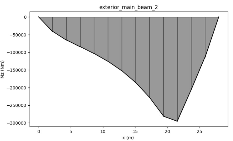
For this section, we refer to an exemplar 28 m super-T bridge (Figure 2). The grillage object is named bridge_28.

Figure 2: 28 m super-T bridge model.

To plot deflection from the displacements DataArray use plot_def(), specifying a grillage member name:

og.plot_def(bridge_28, results, members="exterior_main_beam_2")

Figure 3: Deflected shape of exterior main beam 2.

To plot internal forces from the forces DataArray use plot_force():

og.plot_force(bridge_28, results, member="exterior_main_beam_2", component="Mz")

Figure 4: Bending moment about z axis of exterior main beam 2.

Convenience plotting functions#

For the most common diagrams, convenience wrappers are provided that default to plotting all member groups when no member is specified:

og.plot_bmd(bridge_28, results)          # bending moment diagram (Mz)
og.plot_sfd(bridge_28, results)          # shear force diagram (Fy)
og.plot_def(bridge_28, results)   # vertical deflection (y)

Each returns a list of figures (one per member group). Pass member="interior_main_beam" to plot a single member instead.

Selecting member groups#

The member parameter accepts a string for a single member, or a Members bitflag to plot any combination of groups:

# Plot only longitudinal members
og.plot_bmd(bridge_28, results, member=og.Members.LONGITUDINAL, backend="plotly")

# Combine individual members with |
og.plot_bmd(bridge_28, results,
            member=og.Members.EDGE_BEAM | og.Members.INTERIOR_MAIN_BEAM,
            backend="plotly")

# Plot everything (the default for plotly)
og.plot_bmd(bridge_28, results, member=og.Members.ALL, backend="plotly")

Available individual flags:

Flag	Member name string
`EDGE_BEAM`	`"edge_beam"`
`EXTERIOR_MAIN_BEAM_1`	`"exterior_main_beam_1"`
`INTERIOR_MAIN_BEAM`	`"interior_main_beam"`
`EXTERIOR_MAIN_BEAM_2`	`"exterior_main_beam_2"`
`START_EDGE`	`"start_edge"`
`END_EDGE`	`"end_edge"`
`TRANSVERSE_SLAB`	`"transverse_slab"`

Pre-defined composites: LONGITUDINAL (all four longitudinal types), TRANSVERSE (transverse slab + start/end edges), ALL (everything).

Customising plots#

All plotting functions accept keyword arguments for common customisations:

# Wide figure, values in kN*m, custom title, red with no fill
og.plot_bmd(bridge_28, results,
            member="interior_main_beam",
            figsize=(12, 4),
            scale=0.001,
            title="Bending Moment (kN*m)",
            color="r",
            fill=False)

To compose multi-panel figures, pass an existing matplotlib Axes:

import matplotlib.pyplot as plt
fig, axes = plt.subplots(1, 3, figsize=(18, 4))
og.plot_bmd(bridge_28, results, member="interior_main_beam", ax=axes[0])
og.plot_sfd(bridge_28, results, member="interior_main_beam", ax=axes[1])
og.plot_def(bridge_28, results, member="interior_main_beam", ax=axes[2], color="g")
fig.tight_layout()

The full set of keyword arguments is:

Kwarg	Default	Description
`figsize`	matplotlib default	Figure size in inches `(width, height)`
`ax`	`None`	Existing Axes (matplotlib) or Figure (Plotly) to draw on
`scale`	`1.0`	Multiply values by this factor (e.g. `0.001` for N to kN)
`title`	auto	Custom title string, or `None` to suppress
`color`	`"k"` / `"b"`	Line colour
`fill`	`True`	Shade the area under force diagrams
`alpha`	`0.4`	Fill / trace transparency
`show`	`False`	Call `fig.show()` before returning

Interactive 3D plots (Plotly)#

For interactive rotation — especially useful in Jupyter notebooks — pass backend="plotly":

pip install ospgrillage[gui]   # includes plotly

og.plot_bmd(bridge_28, results, backend="plotly")
og.plot_sfd(bridge_28, results, backend="plotly")
og.plot_def(bridge_28, results, backend="plotly")

Each returns a single Plotly Figure that renders interactively in Jupyter notebooks and in browser windows from the terminal. The figure can be further customised using the standard Plotly API. The GUI auto-detects plotly and uses it by default when available.

Shell contour plots (`plot_srf`)#

For shell_beam models, plot_srf() renders contour plots over the shell mesh. It supports three families of component:

Family	Components	Description
Shell forces	`Vx`, `Vy`, `Vz`, `Mx`, `My`, `Mz`	Element end forces averaged to nodes
Displacements	`Dx`, `Dy`, `Dz`	Nodal translations (x, y, z)
Stress resultants	`N11`, `N22`, `N12`, `M11`, `M22`, `M12`, `Q13`, `Q23`	Section stress resultants averaged from Gauss points

Note

plot_srf requires a shell_beam model. The results Dataset must contain ele_nodes_shell and node_coordinates. Stress resultant components additionally require stresses_shell (generated automatically by ospgrillage ≥ 0.6.0).

Basic usage#

plot_srf takes a results Dataset (not a grillage object) as its first argument:

results = bridge.get_results(save_filename="bridge_results.nc")

# Shell bending moment about the x-axis
og.plot_srf(results, component="Mx")

# Vertical displacement contour
og.plot_srf(results, component="Dy")

# Membrane force N11 (stress resultant)
og.plot_srf(results, component="N11")

Choosing a loadcase#

By default the first loadcase is plotted. Pass loadcase= to select a specific one:

og.plot_srf(results, component="Mx", loadcase="Dead Load")

Shell force components#

Shell element end forces (Vx–Mz) are extracted from forces_shell and averaged at shared nodes:

og.plot_srf(results, "Mx")   # bending moment about x
og.plot_srf(results, "Vy")   # shear force in y
og.plot_srf(results, "Mz")   # torsion

Displacement components#

Displacement contours (Dx, Dy, Dz) are read directly from the nodal displacements array:

og.plot_srf(results, "Dy")                              # vertical deflection
og.plot_srf(results, "Dy", colorscale="Viridis")        # sequential palette

Tip

Use a sequential colorscale like Viridis for displacements (single-sign data) and a diverging colorscale like RdBu_r (the default) for forces and stress resultants (signed data that crosses zero).

Stress resultant components#

Shell section stress resultants are extracted via OpenSeesPy’s eleResponse(tag, "stresses"), which returns 8 values at each of the 4 Gauss points for a 4-node shell element:

Notation	Meaning
`N11`	Membrane force per unit length in local 1-direction
`N22`	Membrane force per unit length in local 2-direction
`N12`	In-plane shear force per unit length
`M11`	Bending moment per unit length about local 2-axis
`M22`	Bending moment per unit length about local 1-axis
`M12`	Twisting moment per unit length
`Q13`	Transverse shear force per unit length in 1–3 plane
`Q23`	Transverse shear force per unit length in 2–3 plane

og.plot_srf(results, "M11")   # plate bending about local 2-axis
og.plot_srf(results, "N11")   # membrane force in local 1-direction
og.plot_srf(results, "Q13")   # transverse shear

Composing shell contours with beam diagrams#

A common workflow is to overlay the beam BMD/SFD on top of a shell contour. Pass the Plotly figure returned by plot_srf as the ax= argument to any beam plot function:

# 1. Create the shell contour (show=False to keep the figure object)
fig = og.plot_srf(results, "Mx", backend="plotly", show=False)

# 2. Create a model proxy for beam plotting
proxy = og.model_proxy_from_results(results)

# 3. Overlay the BMD onto the same figure
og.plot_bmd(proxy, results, backend="plotly", ax=fig)

This works with plot_bmd, plot_sfd, plot_tmd, and plot_def.

Colorscale guidance#

Data type	Recommended colorscale	Why
Forces / moments (`Vx`–`Mz`)	`RdBu_r` (default)	Diverging — highlights sign change
Stress resultants (`N11`–`Q23`)	`RdBu_r` (default)	Diverging — signed data
Displacements (`Dx`, `Dy`, `Dz`)	`Viridis`	Sequential — typically single-sign

og.plot_srf(results, "Mx", colorscale="RdBu_r")     # diverging (default)
og.plot_srf(results, "Dy", colorscale="Viridis")     # sequential
og.plot_srf(results, "N11", colorscale="Plasma")     # alternative sequential

Additional keyword arguments#

Kwarg	Default	Description
`backend`	`"plotly"`	`"plotly"` for interactive 3-D or `"matplotlib"` for 2-D
`colorscale`	`"RdBu_r"`	Plotly colorscale name (or matplotlib `cmap` name)
`show_colorbar`	`True`	Display the colour bar legend
`opacity`	`1.0`	Surface opacity (0–1)
`show`	`True` (plotly) / `False` (mpl)	Display the figure immediately
`ax` / `fig`	`None`	Existing Plotly `Figure` or matplotlib `Axes` to draw on
`title`	auto	Custom title string, or `None` to suppress
`figsize`	`None`	Figure size as `(width, height)` in inches

Using the GUI shell contour tab#

When you open a shell_beam results file in the GUI (File > Open Results (.nc)), a Shell Contour tab appears alongside the BMD, SFD, TMD, and Deflection tabs.

The results panel on the left provides three controls:

Component — select any of the 17 available components (Mx–Mz, Dx–Dz, N11–Q23)
Colorscale — choose from RdBu_r, Viridis, Plasma, Cividis, or Turbo
Overlay — optionally composite a beam diagram (BMD, SFD, TMD, or Deflection) on top of the shell contour

The contour controls are greyed out when a non-contour tab is selected and automatically enabled when you switch to the Shell Contour tab. For non-shell models, the tab and controls are hidden entirely.

Working with results#

Extracting results#

What is an xarray Dataset?#

Extracting the data variables#

Available force and displacement components#

Selecting results by label#

Load combinations#

Load envelopes#

Saving and loading results#

Loading saved results#

Plotting from a saved file#

Viewing results in the GUI#

Plotting results#

Model visualisation#

Post-processing results#

Convenience plotting functions#

Selecting member groups#

Customising plots#

Interactive 3D plots (Plotly)#

Shell contour plots (plot_srf)#

Basic usage#

Choosing a loadcase#

Shell force components#

Displacement components#

Stress resultant components#

Composing shell contours with beam diagrams#

Colorscale guidance#

Additional keyword arguments#

Using the GUI shell contour tab#

Shell contour plots (`plot_srf`)#