Getting Results

For all example code in this page, ospgrillage is imported as og

import ospgrillage as og

Extracting results

After analysis, results are obtained using get_results().

all_result   = example_bridge.get_results()
patch_result = example_bridge.get_results(load_case="patch load case")

The first call returns results for every load case; the second filters to one.

What is an xarray Dataset?

The returned object is an xarray Dataset — think of it as a multi-dimensional, labelled table. Rather than accessing data by integer index (row 3, column 7), you access it by name (Loadcase="Barrier", Component="Mz_i"). This makes result queries self-describing and much less error-prone.

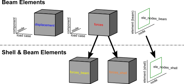
The Dataset contains three named data variables:

Variable	Axes (dimensions)	Contents
displacements	Loadcase × Node × Component	Translations (dx, dy, dz) and rotations (theta_x/y/z) at each node
forces	Loadcase × Element × Component	Internal forces (Mx, My, Mz, Vx, Vy, Vz) at each element end (_i, _j)
ele_nodes	Element × Nodes	Which node tags (i, j) belong to each element

For a Shell & Beam Elements — shell_beam, forces are split into forces_beam / forces_shell and element connectivity into ele_nodes_beam / ele_nodes_shell.

Printing all_result shows the structure:

<xarray.Dataset>
Dimensions:        (Component: 18, Element: 142, Loadcase: 5, Node: 77, Nodes: 2)
Coordinates:
  * Component      (Component) <U7 'Mx_i' 'Mx_j' 'My_i' ... 'theta_y' 'theta_z'
  * Loadcase       (Loadcase) <U55 'Barrier' ... 'single_moving_point at glob...'
  * Node           (Node) int32 1 2 3 4 5 6 7 8 9 ... 69 70 71 72 73 74 75 76 77
  * Element        (Element) int32 1 2 3 4 5 6 7 ... 136 137 138 139 140 141 142
  * Nodes          (Nodes) <U1 'i' 'j'
Data variables:
    displacements  (Loadcase, Node, Component) float64 nan nan ... -4.996e-10
    forces         (Loadcase, Element, Component) float64 36.18 -156.9 ... nan
    ele_nodes      (Element, Nodes) int32 2 3 1 2 1 3 4 ... 32 75 33 76 34 77 35

Each line of Coordinates lists the labels along one dimension. Loadcase lists every load case name; Component lists every result quantity; Node and Element list the integer tags from the OpenSees model.

Figure 1 illustrates the overall dataset structure.

Extracting the data variables

disp_array = all_result.displacements  # nodal displacements & rotations
force_array = all_result.forces        # element end forces
ele_array   = all_result.ele_nodes     # element→node connectivity

Available force and displacement components

To see the full list of component labels:

force_array.coords['Component'].values

array(['Mx_i', 'Mx_j', 'My_i', 'My_j', 'Mz_i', 'Mz_j', 'Vx_i', 'Vx_j',
       'Vy_i', 'Vy_j', 'Vz_i', 'Vz_j', 'dx', 'dy', 'dz', 'theta_x',
       'theta_y', 'theta_z'], dtype='<U7')

Suffix _i / _j denotes the start / end node of the element respectively.

Selecting results by label

Use xarray’s .sel() to pick results by name, and .isel() to pick by integer position:

# All nodes, one component
disp_array.sel(Component='dy')

# One load case, one node
disp_array.sel(Loadcase="patch load case", Node=20)

# One load case, several elements
force_array.sel(Loadcase="Barrier", Element=[2, 3, 4])

# One component across all load cases
force_array.sel(Component='Mz_i')

For results from a Moving load, each increment is stored as a separate load case named automatically as "<load name> at global position [x,y,z]". You can select these by full name or by position:

# Select by the auto-generated name
by_name  = force_array.sel(Loadcase="patch load case at global position [0,0,0]")
# Select by integer index (0 = first increment)
by_index = force_array.isel(Loadcase=0)

Note

For information on the full range of indexing and selection operations available on DataArrays, see the xarray indexing documentation.

Getting combinations

Load combinations are computed on the fly in get_results() by passing a combinations dictionary: keys are load case name strings and values are load factors. ospgrillage multiplies each load case by its factor and sums the results.

comb_dict   = {"patch_load_case": 2, "moving_truck": 1.6}
comb_result = example_bridge.get_results(combinations=comb_dict)
print(comb_result)

<xarray.Dataset>
Dimensions:        (Component: 18, Element: 142, Loadcase: 3, Node: 77, Nodes: 2)
Coordinates:
  * Component      (Component) <U7 'Mx_i' 'Mx_j' 'My_i' ... 'theta_y' 'theta_z'
  * Node           (Node) int32 1 2 3 4 5 6 7 8 9 ... 69 70 71 72 73 74 75 76 77
  * Element        (Element) int32 1 2 3 4 5 6 7 ... 136 137 138 139 140 141 142
  * Nodes          (Nodes) <U1 'i' 'j'
  * Loadcase       (Loadcase) <U55 'moving_truck at global position [2...'
Data variables:
    displacements  (Loadcase, Node, Component) float64 nan nan ... 0.0 7.688e-05
    forces         (Loadcase, Element, Component) float64 36.18 -156.9 ... nan
    ele_nodes      (Loadcase, Element, Nodes) int32 6 9 3 6 ... 228 102 231 105

When a combination mixes static and moving load cases, the factored static load case is added to each increment of the moving load.

Getting load envelope

A load envelope finds the maximum (or minimum) of a chosen result component across all load cases. Use create_envelope() to build an Envelope object, then call .get():

envelope = og.create_envelope(ds=comb_result, load_effect="dy", array="displacements")
disp_env = envelope.get()
print(disp_env)

By default get() returns, for each node, the name of the load case that produced the maximum value of dy:

<xarray.DataArray 'Loadcase' (Node: 77, Component: 18)>
array([[nan, nan, nan, ...,
        'single_moving_point at global position [2.00,0.00,2.00]', ...],
       ...],
      dtype=object)
Coordinates:
  * Component  (Component) <U7 'Mx_i' 'Mx_j' 'My_i' ... 'theta_y' 'theta_z'
  * Node       (Node) int32 1 2 3 4 5 6 7 8 9 10 ... 69 70 71 72 73 74 75 76 77

For more options see create_envelope().

Getting specific properties of model

Node

Use get_nodes() to retrieve node information from the model.

Element

Use get_element() to query element properties and tags from the model.

Plotting results

Current limitation of OpenSees visualization modules

OpenSeesPy’s visualization modules (vfo and opsvis) require the model to be active in the OpenSees model space. Results retrieved via get_results() are stored in an xarray Dataset and cannot be fed back to these modules for multi-load-case plotting. Additionally, neither module supports enveloping across multiple incremental load cases.

For single-load-case inspection only, opsvis can be used directly after analysis:

og.opsv.section_force_diagram_3d('Mz', {}, 1)

Note

opsv only works for model templates beam_only and beam_link. Shell model plotting is not supported as of ospgrillage version 0.1.0.

ospgrillage post-processing module

For multi-load-case or moving load results, ospgrillage includes a dedicated post-processing module.

Note

The plotting functions of the post-processing module are at alpha development stage. As of version 0.1.0 they are sufficient for plotting components from xarray DataSets.

For this section, we refer to an exemplar 28 m super-T bridge (Figure 2). The grillage object is named bridge_28.

To plot deflection from the displacements DataArray use plot_defo(), specifying a grillage member name:

og.plot_defo(bridge_28, results, member="exterior_main_beam_2", option="nodes")

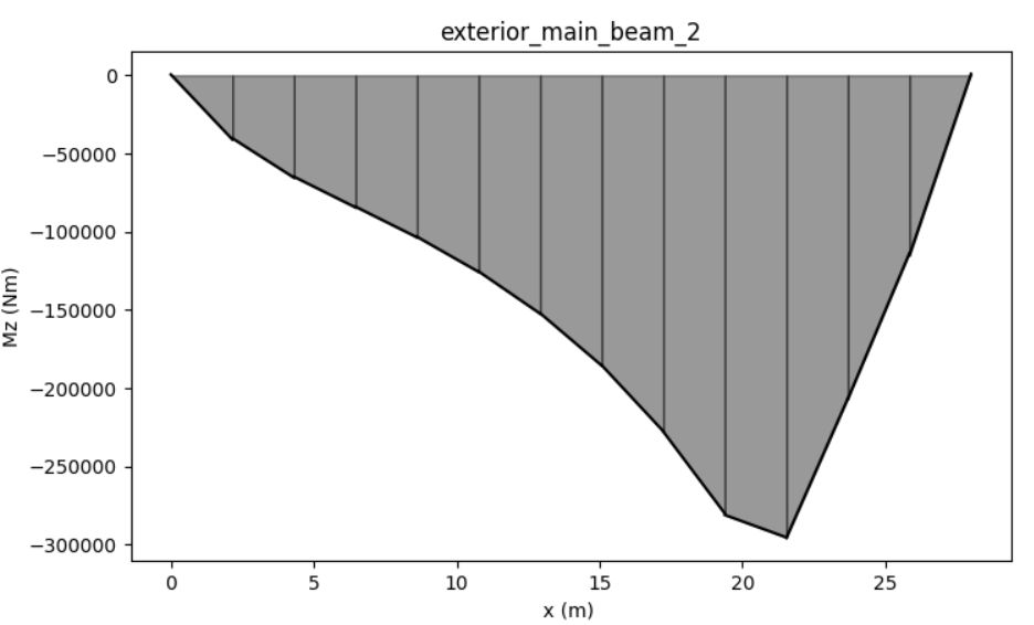
To plot internal forces from the forces DataArray use plot_force():

og.plot_force(bridge_28, results, member="exterior_main_beam_2", component="Mz")